From Tokens to Tensors: An Engineer's Deep Dive into LLM Inference Performance
Moving beyond the API: How understanding the silicon-level processing can shave seconds off your inference latency

As engineers, we often interact with Large Language Models (LLMs) via a simple POST request to an API endpoint. We send a string, and a few hundred milliseconds later, we get a response. But for those building production-grade AI applications, the “black box” approach isn’t enough.
To optimize for latency (TTFT), throughput (TPS), and cost, we have to peel back the layers of the Transformer architecture. We need to understand why the decoding phase is a memory hog, how tokenization can break your logic, and why the KV cache is the most important piece of memory you’re currently managing.
The Architecture Debate: Why “Decoder-Only” Won
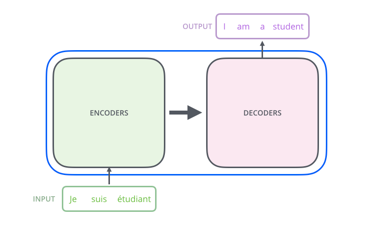
When the Transformer was first introduced in the Attention is All You Need paper, it was a symmetrical beast: an Encoder to understand the input and a Decoder to generate the output.
However, the industry has largely converged on the Decoder-only architecture (think GPT-4, Llama 3, and Mistral). Why?
Encoders (e.g., BERT, RoBERTa): These use “bi-directional” attention. They look at every word in a sentence simultaneously to create a dense representation (embedding). They are king for classification and NER but lack the fluid generative capabilities of their counterparts.
Encoder-Decoders (e.g., T5, BART): These were the standard for translation. The encoder processes the source language, and the decoder generates the target.
Decoder-Only: These use “causal” or “masked” attention. They only look at previous tokens in a sequence. Through massive scaling, we’ve discovered that these models don’t actually need a separate encoder. They can derive the context of a prompt and generate a response within the same mathematical framework. This simplifies the inference pipeline, making it easier to scale on modern GPU clusters.
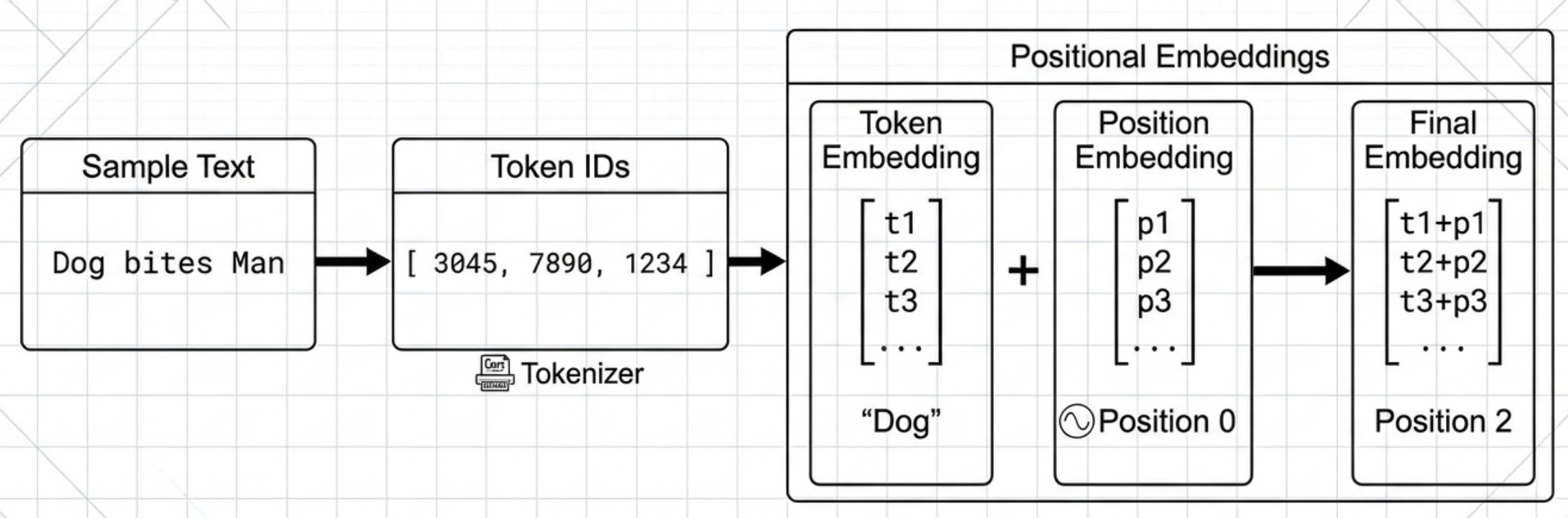
Tokenization: The “Lossy” Bridge to Math
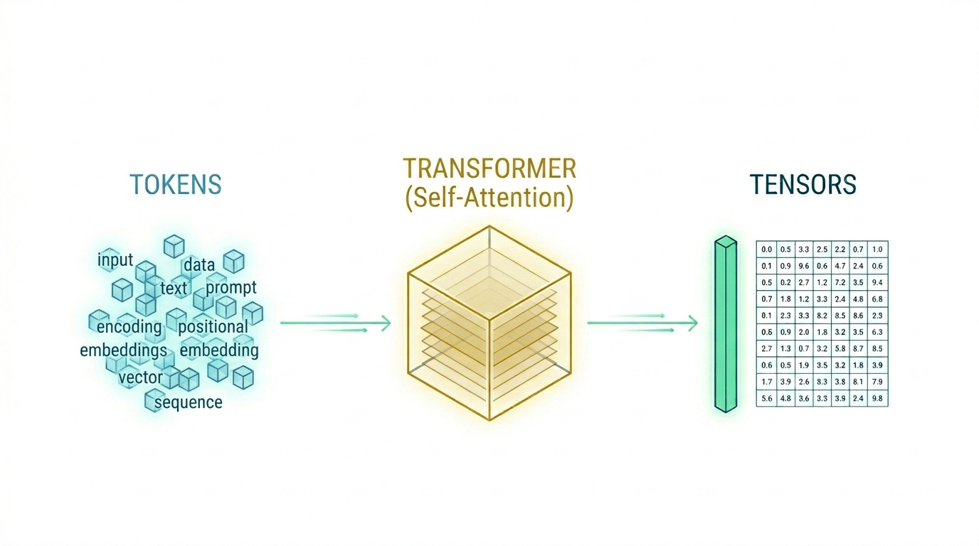
LLMs do not process strings; they process tensors of floating-point numbers. The first engineering hurdle is Tokenization.
Subword Tokenization vs. Character Level
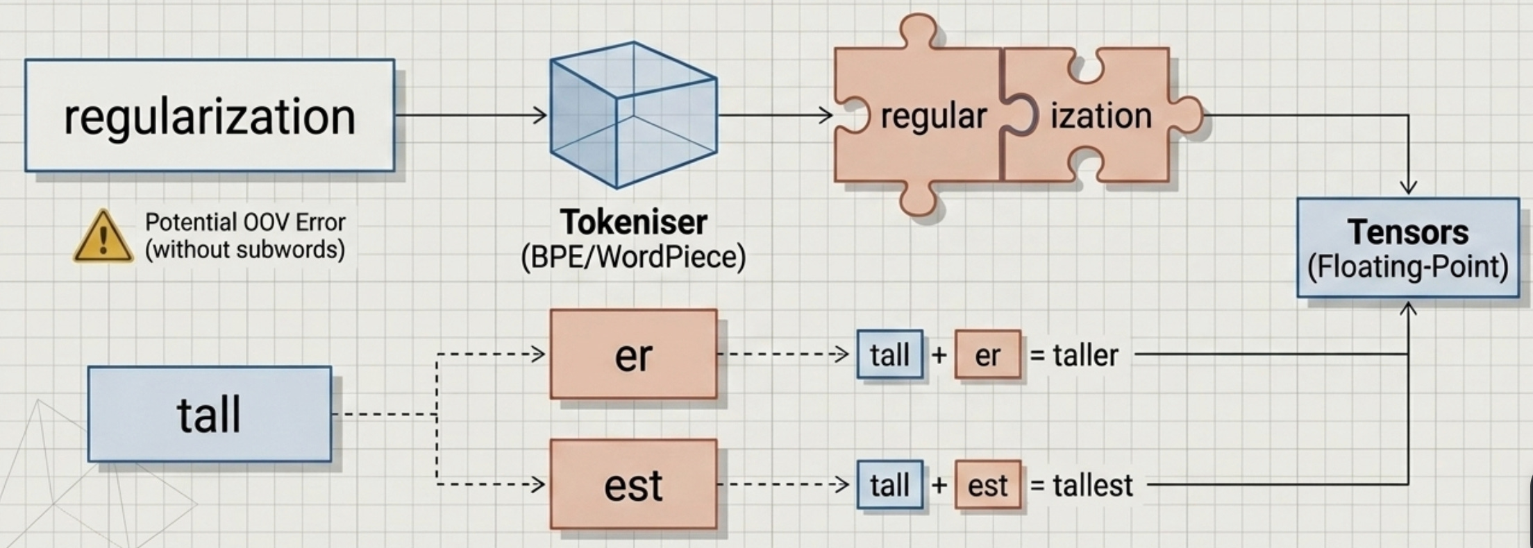
A naive approach would be to assign an integer to every word. But dictionaries are infinite, and typos are common. If your model encounters a word it hasn’t seen (an “Out of Vocabulary” or OOV error), the system fails.
Modern LLMs use Subword Tokenization (like Byte-Pair Encoding or WordPiece). This breaks text into the smallest meaningful chunks.
Example: The word regularization might be tokenized as
[regular,ization].Example: The suffix er is a common token. This allows the model to
handletall, tallerandtallest byreusingtheeandest tokens, keeping the vocabulary size manageable (usually between 32k and 128k tokens).
The Engineer’s Token Tax
As an engineer, you must remember that 1 token ~= 0.75 words (or roughly 4 characters in English). However, tokenizers are model-specific. If you use a Llama-3 tokenizer to estimate the cost for a GPT-4o request, your math will be wrong. This is particularly critical when building “RAG” (Retrieval-Augmented Generation) systems where you are stuffing thousands of tokens of context into a prompt, every token counts toward your rate limits and your bill.
Embeddings and the High-Dimensional Galaxy
Once we have our list of token IDs, we move to the Embedding Layer.
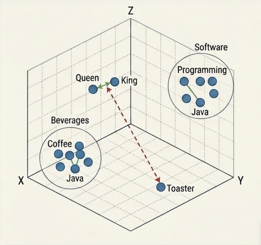
Imagine a map. On a 2D map, “Paris” and “London” are close together. In an LLM, we use a “map” with thousands of dimensions. Each token ID is mapped to a vector in this high-dimensional space.
Semantic Proximity is the goal here. The vector for Queen should be closer to King than it is to Toaster. During the training phase, the model learns these relationships. In inference, these “static” embeddings are fed into the Transformer blocks where Self-Attention transforms them into Contextual Embeddings.
This is how the model knows that the word “Java” in a blog about programming is different from “Java” in a blog about coffee. The surrounding vectors pull the “Java” vector toward the “Programming” cluster in that high-dimensional space.
Positional Embeddings: Teaching the Model to Read
A massive quirk of the Transformer architecture is that it is “permutation invariant.” Because the attention mechanism calculates the relationship between all tokens in a set simultaneously, the model has no innate way of knowing if “Dog bites Man” or “Man bites Dog.”
To solve this, we use Positional Embeddings. This involves injecting information about the specific position of each token in the sequence into the vector.
Sinusoidal Embeddings: The original method used sine and cosine functions of different frequencies.
RoPE (Rotary Positional Embeddings): Used by modern models like Llama. Instead of adding a vector, it rotates the embedding in the high-dimensional space. This allows for better “extrapolation,” meaning the model can sometimes handle sequences longer than those it was trained on.
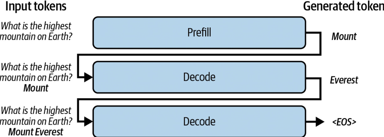
The Two Phases of Inference: Prefill and Decode
This is where the engineering complexity peaks. LLM inference is not a single, monolithic task; it is a tale of two phases with completely different hardware requirements.
Phase 1: The Prefill (Compute-Bound)
When you send a prompt, the model first processes the entire input. This is the Prefill Phase.
What happens: The model takes all “N” tokens of your prompt and calculates their hidden states in parallel.
The Bottleneck: This is compute-bound. It depends on how many TeraFLOPS your GPU can push.
The Metric: This phase determines your Time to First Token (TTFT). If you have a massive prompt, the prefill takes longer, but modern GPUs are highly optimized for this parallel matrix multiplication.
Phase 2: The Decode (Memory-Bound)
Once the first token is generated, the model enters the Decoding Phase. Because LLMs are autoregressive, they generate one token at a time. To generate token #51, the model must look at tokens #1 through #50.
What happens: The model does a single forward pass for one single token.
The Bottleneck: This is memory-bound. You aren’t limited by how fast the GPU can calculate; you are limited by how fast the GPU can move the model weights and the “KV Cache” from VRAM to the processing cores.
The Metric: This determines your Tokens Per Second (TPS).
The KV Cache: Solving the Quadratic Problem
The “Self-Attention” mechanism in Transformers has a major flaw: its computational cost grows quadratically O(n^2) with the sequence length. If you don’t optimize this, generating the 2,000th token would require re-calculating the attention for all 1,999 previous tokens.
To solve this, we use the KV (Key-Value) Cache.
We store the previously calculated “Key” and “Value” vectors in the GPU’s VRAM. When it’s time to generate the next token, the model simply fetches these from the cache instead of recomputing them.
PagedAttention and vLLM
Storing this cache is expensive. For a large model with a long context, the KV cache can consume tens of gigabytes of VRAM. Historically, this required contiguous memory, which led to massive fragmentation (the “OOM” or Out of Memory error we all dread).
The breakthrough came with PagedAttention (implemented in frameworks like vLLM). It borrows a concept from Operating Systems: virtual memory paging. It breaks the KV cache into small, non-contiguous blocks. This allows for:
Near-zero memory waste.
Continuous Batching: Processing multiple requests at once even if they finish at different times.
Prefix Sharing: If ten users are asking questions about the same long document, the model only stores the KV cache for that document once, saving massive amounts of VRAM.
The “Hidden” Logic: Sampling and Temperature
After the model does its math, it doesn’t actually output a word. It outputs a Logits vector, a list of probabilities for every single token in its vocabulary.
If the vocabulary is 50,000 words, the model says: “There is a 40% chance the next word is ‘Apple’, a 20% chance it’s ‘Banana’, and a 0.001% chance it’s ‘Nuclear’.”
Engineers guide this selection using Sampling Parameters:
Temperature: High temperature flattens the probability distribution (making the “Nuclear” option more likely), leading to more creative or “hallucinatory” text. Low temperature (approaching 0) makes the model “greedy,” always picking the #1 choice.
Top-P (Nucleus Sampling): The model only considers the smallest set of tokens whose cumulative probability exceeds ‘P’.
Top-K: The model only considers the top 'K’ most likely tokens.
The Multimodal Future
The text you provided mentions that modern LLMs are becoming multimodal. For an AI engineer, this means the inference pipeline is getting more complex. We aren’t just tokenizing text anymore; we are using Vision Encoders (like CLIP) to turn images into patches. These patches are then mapped into the same embedding space as our text tokens.
Whether the input is a JPEG or a string of Python code, it eventually becomes a sequence of vectors that the Transformer processes using the same attention mechanism. This is why “Large Language Models” is becoming a bit of a misnomer, they are increasingly “Large Multimodal Action Models.”
Final Thoughts for the engineers
Understanding the inference pipeline is the difference between a prototype that works on your local machine and a production system that scales to thousands of users.
Key Takeaways:
Optimize your Prefill: Use shorter prompts or KV-cache sharing to reduce TTFT.
Watch your VRAM: The KV cache is your biggest bottleneck for high-concurrency systems.
Choose the right runtime: Don’t just run raw PyTorch in production. Use specialized inference engines like
vLLM,TGI(Text Generation Inference), orTensorRT-LLM.
What’s your current stack for LLM inference? Are you hitting memory limits or compute limits? Let’s troubleshoot in the comments below.
References
PagedAttention & vLLM: Kwon, W., et al. (2023). “Efficient Memory Management for Large Language Model Serving with PagedAttention.” The foundational paper for the vLLM project that revolutionized KV cache management.
Disaggregated Inference: Microsoft Research (2024). “Splitwise: Efficient Generative LLM Inference Using Phase Splitting.” A key paper discussing the physical separation of Prefill and Decode phases.
Jay Alammar’s “The Illustrated Word2vec”: jalammar.github.io. One of the best visual explanations of how high-dimensional word embeddings work.
The Illustrated Transformer: jalammar.github.io. A visual breakdown of the encoder-decoder mechanics that paved the way for modern LLMs.